Entrainment Effects in Turbulent Boundary Layers
Ph.D Thesis
Guillem Borrell i Nogueras
September 7th. 2015
Financial and material support
- European Research Council

- Spanish Ministry of Economy

- The PRACE Initiative.

- DoE INCITE Program

Turbulent boundary layer

A vanilla boundary layer.

- No external pressure gradients.
- The solid boundary is perfectly flat.
- Incompressible.
- Over a perfectly smooth wall.
Adverse-pressure-gradient boundary layer.

Atmospheric boundary layer.

Boundary Layer over a rough surface.

How does roughness affect to turbulence in a boundary layer?
\( u^+ = u / u_\tau \), \( y^+ = \nu y / u_\tau \). Rough: ( \( \color{red}{-}\) ). Smooth:( \( \color{blue}{- -}\) )


Townsend's wall similarity hypothesis.
- If scale separation is sufficient ( \( \delta_{99} >> \nu/u_\tau \) ).
- If roughness elements do not interact with the logarithmic layer directly ( \(k^+ < 100, \delta_{99}/k > 40 \) ).
The effect of the roughness is contained within a roughness sublayer with a thickness proportional to \( k \).
\( u_\tau \) is a scaling parameter between rough- and smooth-wall boundary layers, that are similar above the roughness sublayer.
Sufficient scale separation


\( \delta_{99}^+=1500 \). Log layer from \( y^+=100 \) to \( y/\delta_{99} = 0.2 \)
Characteristic roughness height k


Approximate limit of \( k^+ = 100, \delta_{99}/k = 40 \).
Early corrections to the theory
It was mostly accepted, but some experiments (e.g. Antonia 1972) found some communication between the wall and the outer region.
- Higher wall-normal velocity fluctuations.
- Different Reynolds shear stress profile.
- Intense bursting that reaches the edge of the BL.
Krogstad & Antonia (1994)
Structure of turbulend boundary layers on smooth and rough walls.
- Rough-wall boundary layer at \( \delta_{99}^+ \sim 4000 \)
- Woven mesh roughness with \( \delta_{99}/ k \sim 50, k^+ = 46 \)
- High equivalent sand roughness \( \color{blue}{k_s^+}\color{black}{ \sim 331} \)
- Significantly shorter correlation lengths.
- Reduced anisotropy.
- Correlation between the structure of the flow and the arrangement of the roughness elements
Later works.
- Different correlation lenghts, but not like in K&A('94).
- Differences in velocity fluctuations, Reynolds stresses...
- All those effects are not equally observed in channels.
The relationship between friction and entrainment.
\[ \int_0^\infty \langle\partial_t u + \boldsymbol{u}\cdot \nabla u = -\nabla p + \nu \nabla^2 \boldsymbol{u} \rangle_t\ \mbox{d}y \]
\[ \theta = \int_0^\infty \frac{\langle u \rangle}{U_\infty} \left ( 1 - \frac{\langle u \rangle}{U_\infty} \right)\ \mbox{d}y \]
\[ \frac{\mbox{d}\theta}{\mbox{d}x} = \frac{c_f}{2} = \frac{\color{red}{u_\tau^2}}{U_\infty^2} \]
How does roughness entrainment affect to turbulence
in a boundary layer?
The wall similarity hypothesis is assumed at this point. If entrainment \( \sim \) roughness will be discussed a posteriori.
A DNS to study enhanced entrainment.

Chapter 2. Borrell, Sillero & Jiménez (C and F 2013)
Near-wall force
\[ \frac{\partial u}{\partial t} + \boldsymbol{u} \cdot \nabla u = -\frac{\partial p}{\partial x} + \nu\nabla^2 \boldsymbol{u} - \color{red}{u_0}\color{blue}{g}/\color{green}{T} \] \[ \tau_w = u_\tau^2 = \nu \left. \frac{\partial \langle u \rangle} {\partial y} \right|_{y=0} + \frac{1}{\color{green}{T}} \int_0^\infty \color{red}{u_0} \color{blue}{g}\ \color{black}{\mbox{d}y} \] \[ \color{red}{u_0(x,y,t) = \langle u(x,y,z,t) \rangle_z} \] \[ \color{blue}{g = \frac{1}{2} \left(1 -\tanh \left( \frac{y-y_0}{y_1} \right)\right) }\] \[ \color{green}{T = \frac{1}{\tau_w^0}\int_0^\infty u_0 g\ \mbox{d}y} \]\( \tau_w \simeq 1.75 \tau_w^0 \), \( k^+=25 \), \( \delta_{99}/k=50-70 \), \( k_s^+\simeq 70 \)
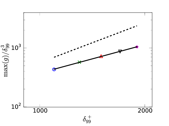
Comparison between rough- and smooth-wall boundary layers.
| Case | Range \( \delta_{99}^+ \) | Comp. \( \delta_{99}^+ \) | Symbol |
|---|---|---|---|
| Present | 800-1650 | 1500 | \( \color{red}{Solid} \) |
| Sillero et al. | 1000-2000 | 1500 | \( \color{blue}{Dashed} \) |
| Del Álamo et al. | 950 | 950 | \( \color{magenta}{-\square-} \) |
| Hoyas & Jiménez. | 2000 | 2000 | \( \color{green}{-\triangledown-} \) |
The forcing causes a step change in the friction coefficient. At \( \delta_{99}^+=1500 \) it has recovered from it.
Velocity and pressure fluctuations


Turbulent kinetic energy


— ‐, \( \alpha g(y^+) \)
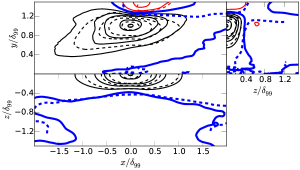
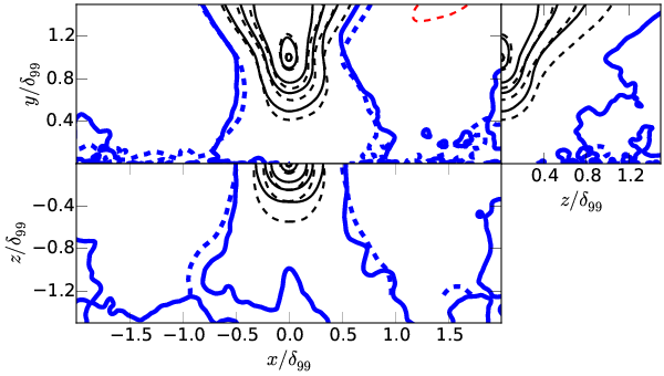
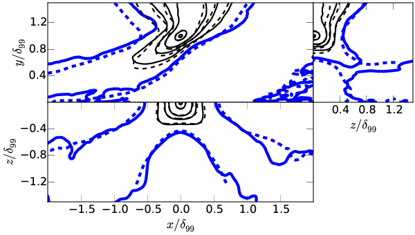
Velocity autocorrelations
For each component of velocity \( u_i \) and point in space \( \boldsymbol{x^\prime} \)
\[ C_{u_iu_i} = \frac{E[ (u_i(\boldsymbol{x}) - \langle u_i(\boldsymbol{x}) \rangle) (u_i(\boldsymbol{x^\prime}) - \langle u_i(\boldsymbol{x^\prime}) \rangle) ]}{\sigma(u_i(\boldsymbol{x})) \sigma(u_i(\boldsymbol{x^\prime}))} \]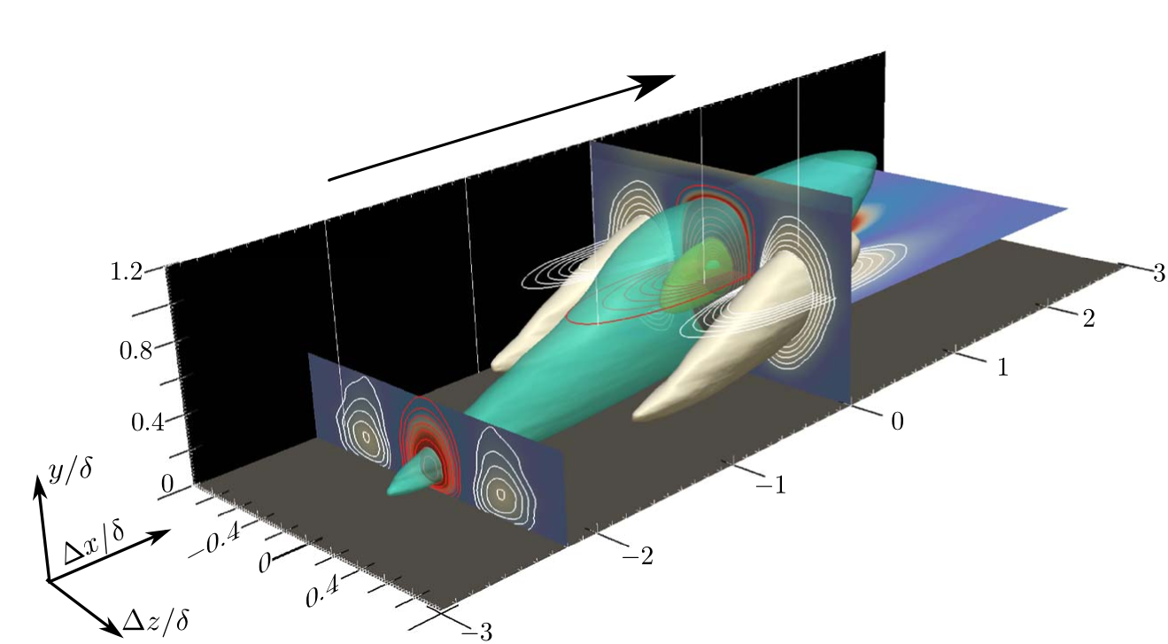
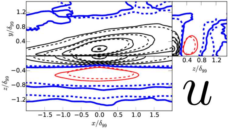
From Sillero et al. (PoF 2014)
\( y^\prime/\delta_{99}=0.2 \)
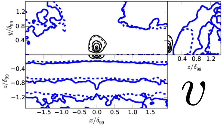
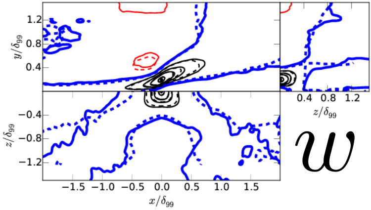
\( y^\prime/\delta_{99}=0.6 \)
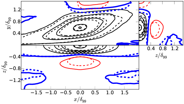
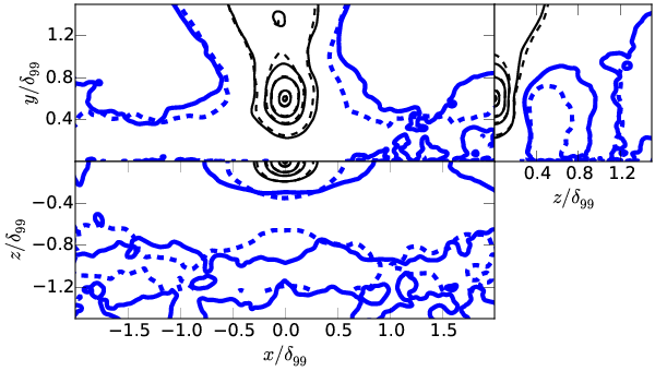
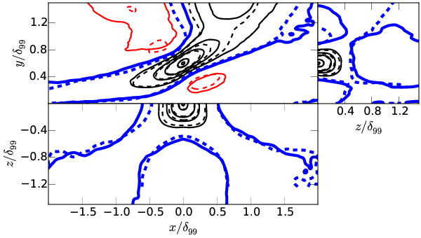
\( y^\prime/\delta_{99}=1.0 \)
Conclusions at this point

Entrainment may be the cause for the differences produced by ``roughness´´ beyond the logarithmic layer.
THE END?
But we do not know very much about entrainment in boundary layers, and about the outer region in general.
\[ \frac{\mbox{d}\theta}{\mbox{d}x}= \frac{u_\tau^2}{U_\infty^2} \]- How does the turbulent motion interact with the irrotational free stream?
- What is the actual mechanism of entrainment?
- Does entrainment depend on the entrainment rate?
- Does entrainment occur identically in BL than in other turbulent external flows?
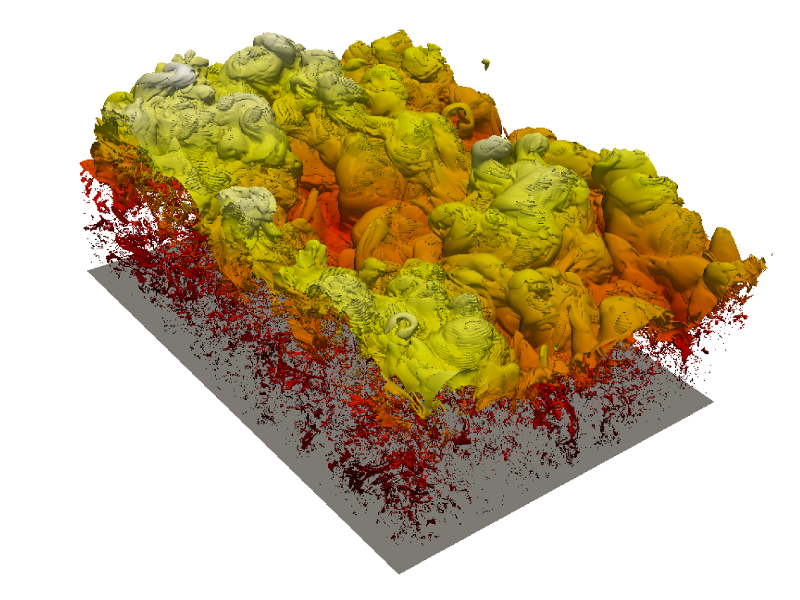
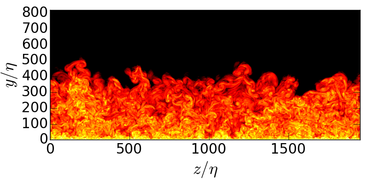
Entrainment and the T/NT interface
\( \omega = | \boldsymbol{\omega} | \), \( \nabla^2
\boldsymbol{u} = -\nabla \wedge \boldsymbol {\omega} \)
\(
\color{blue}{\omega(x,y,z,t) = \omega_0} \) is the
T/NT.
Data: Sillero et al. (2013,2014). NO FORCING.
The intermittent region.
Average properties of the T/NT interface.
\[ \langle \omega^+\rangle \simeq \left( \kappa y ^+ \right) ^{-1/2}\ ( -\circ -) \] \[ \nu {\omega^\prime}^2 \simeq -\langle uv\rangle \frac{\partial \langle u \rangle}{\partial y} \simeq \frac{u_\tau^3}{\kappa y} \] \[ \color{red}{\omega^*} \color{black}{= \omega} \color{blue}{(\delta_{99}^+)^{1/2} \nu /u_\tau^2} \color{black}{=} \color{blue}{(\delta_{99}^+)^{1/2}} \color{black}{\omega^+} \]- Range of possible thresholds \( \omega_0 \).
- Averaged properties give no information about the features of the T/NT interface.
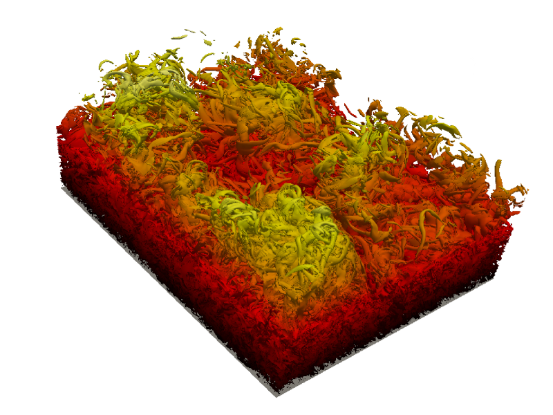
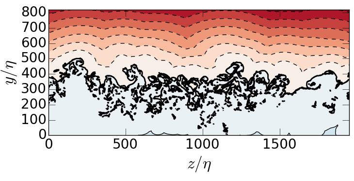
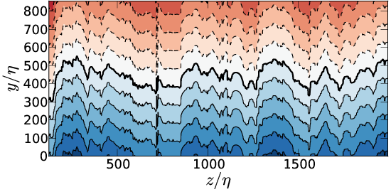
Geometrical complexity of the interface.

Redefine the T/NT as cleaned vorticity isosurface. Only the largest component of \( \omega(x,y,z,t) = \omega_0 \) is relevant.
Conditional analysis of the T/NT layer
- The region within the turbulent side that is visibly affected by the presence of non-turbulent flow.
- Describe the properties of the flow using the T/NT interface as a reference frame
- The goal is to understand the interaction between the turbulent and the non-turbulent flow.
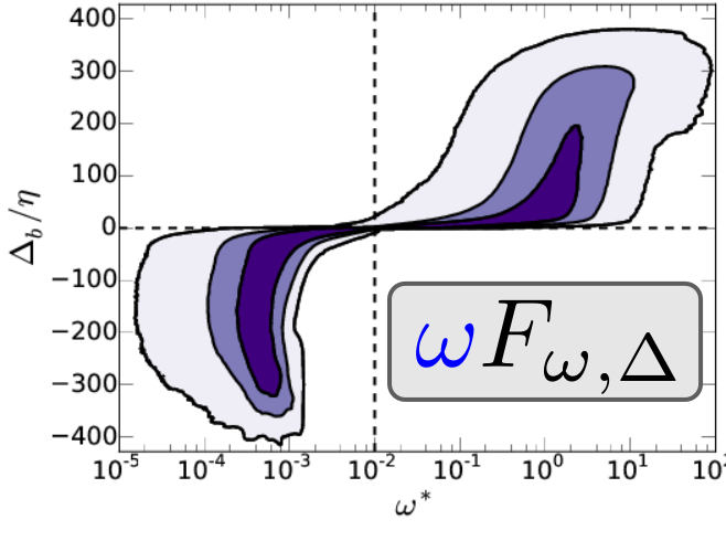
- \( \omega^* \) (but other scalars will be analyzed) and a conditional distance \( \Delta \)
But what distance?


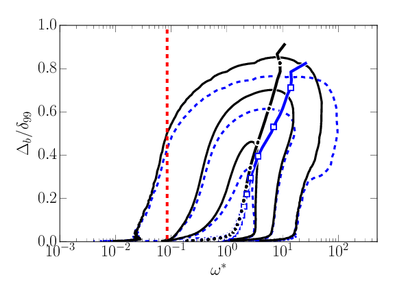
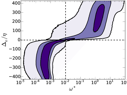
Joint PDF of \( \omega \) and \( \Delta_b \), \( F_{\omega,\Delta_b} \)
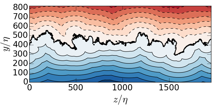
For \(\delta_{99}^+ = 1000-1900\) and \(\omega_0^* = 0.01-0.5\)
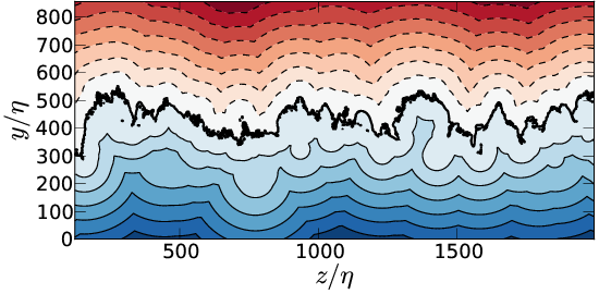
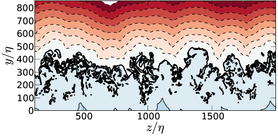
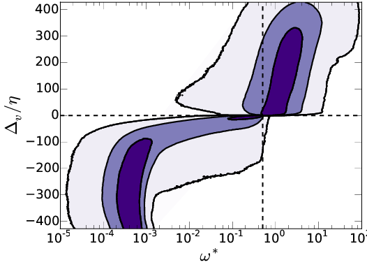
The T/NT as the reference frame.
- \( \Gamma_{\omega,y} \) and \( F_{\omega,\Delta} \) are similar quantities. The difference is the reference frame.
- \( \Gamma_{\omega,y} = F_{\omega,\Delta} \) if \( \omega(x,y,z,t)= \omega_0 \) was \( y = 0 \).
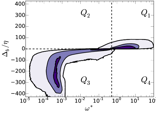
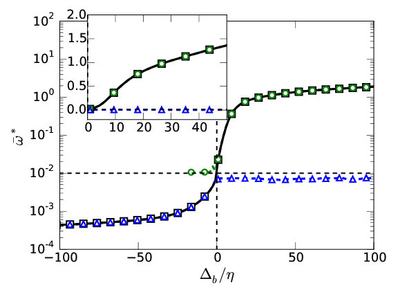
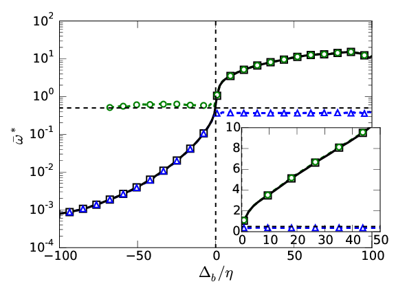
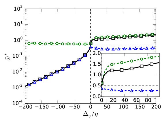
Left \( \omega_0^*=0.01 \), right \( \omega_0^*=0.5
\). Cont:[50%, 90%, ~100%]
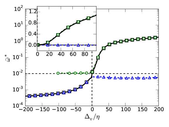
\(\overline{ \omega}
(\Delta) \): \( Q_1 + Q_2 \) \( \color{black}{\square}\), \(
Q_1\) \( \color{green}{\bigcirc} \), \( Q_2 \) \(
\color{blue}{\triangle} \)
The T/NT interface layer.
Three distinct zones.
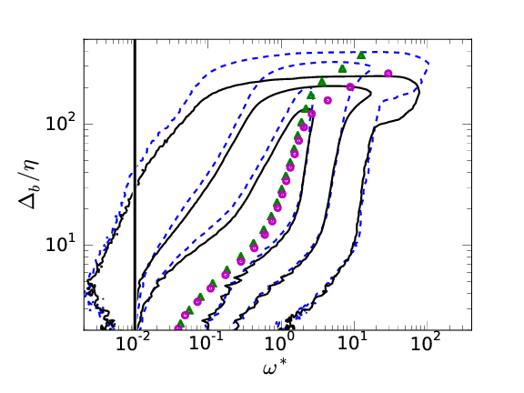
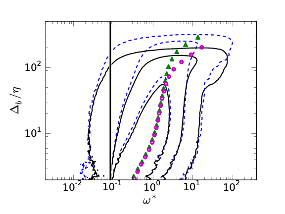
Left: \( \omega_0^*=0.01\ \). Right: \( \omega_0^*=0.09\ \). Cont.:[50%, 90%, 99%] . \( \delta_{99}^+=1100 (\overline{\omega}^*: \color{magenta}{\bullet} \color{black}{}), \color{blue}{1900}\color{black}{} (\overline{\omega}^*:\color{green}{\blacktriangle} \color{black}{} ) \)
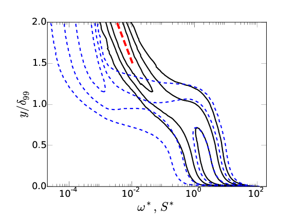
The interface layer
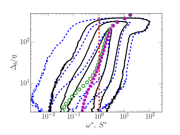
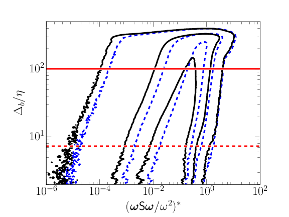
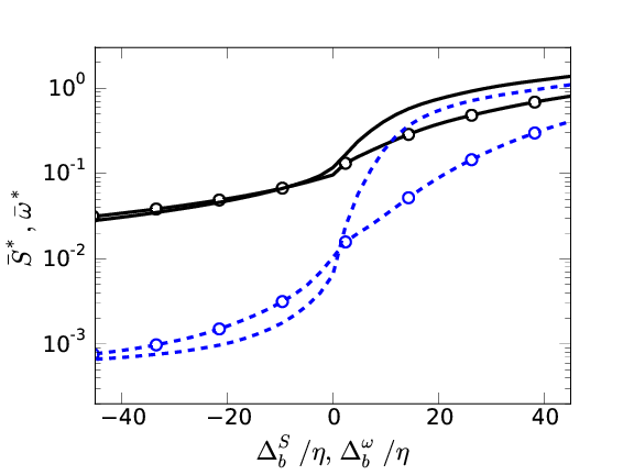
Vorticity interface at \( \omega_0^*=0.01 \). Left: \( \omega^*F_{\omega^*,\Delta_b}\ (\color{blue}{-\ -}\color{black}{)} \), \( S^*F_{S^*,\Delta_b}\ (\color{black}{-}) \), \( \overline{\omega} (\color{green}{\bigcirc}\color{black}{)} \), \( \overline{S} (\color{magenta}{\bullet}\color{black}{)} \). Right: \( \chi^* = (|\boldsymbol{\omega} \boldsymbol{\mathsf{S}} \boldsymbol{\omega} | /\omega^2)^*\), \( \chi^*F_{\chi^*,\Delta_b}\), stretching \( (\color{blue}{-\ -}\color{black}{)} \), compression \( (-) \)
Portrait of entrainment.
- Geometrical complexity is relevant.
- The T/NT interface layer:
- Thin ( \(20\eta, \omega^*=0.01-1 \) )
- Strong vorticity gradient.
- Other quantities are turbulent.
- Beyond the T/NT layer, no influence is measured.
- \( \Delta_b \) Is a good tool to study entrainment.
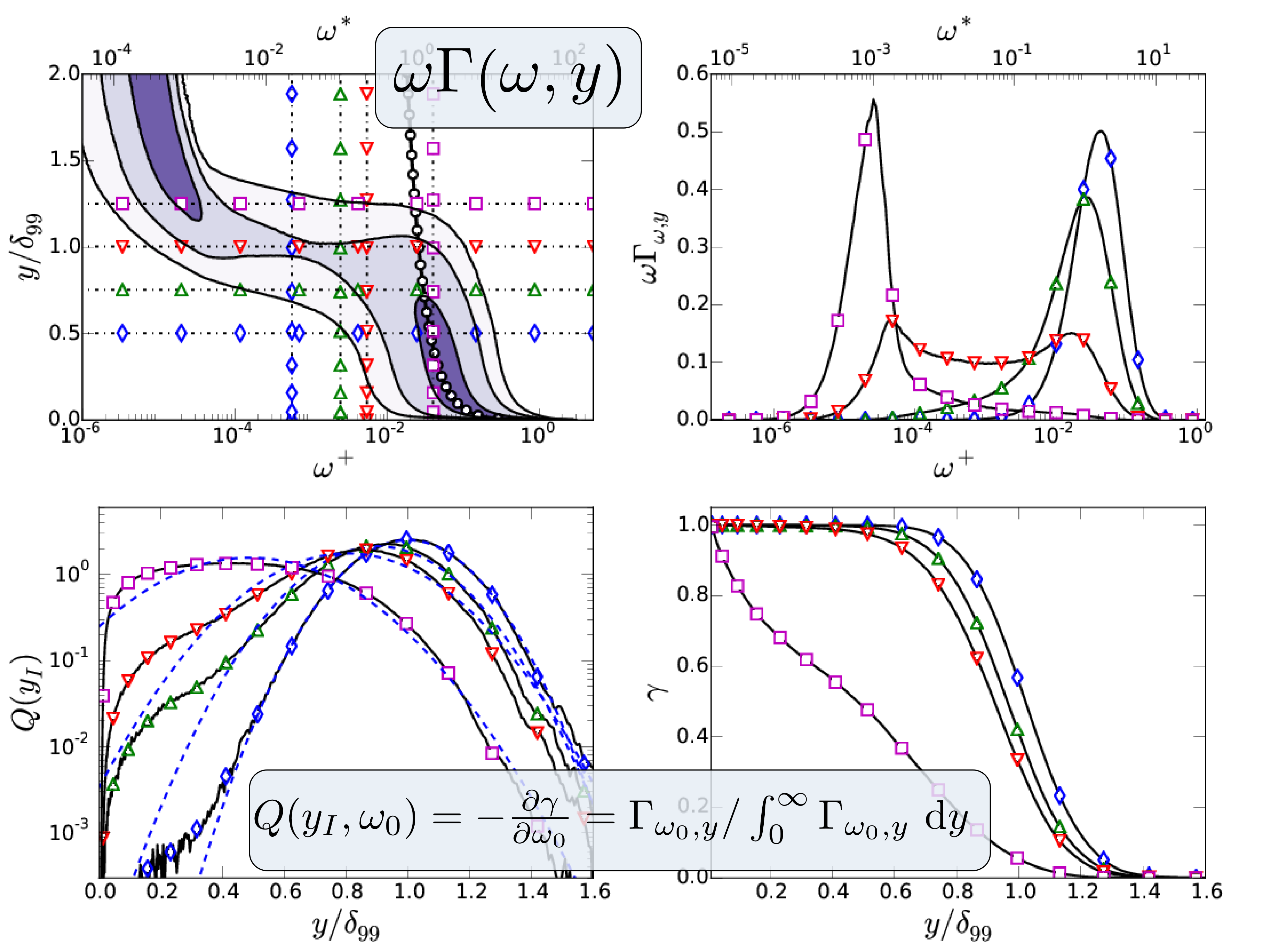
How does enhanced entrainment affect to turbulence in a boundary layer?
From the wall.
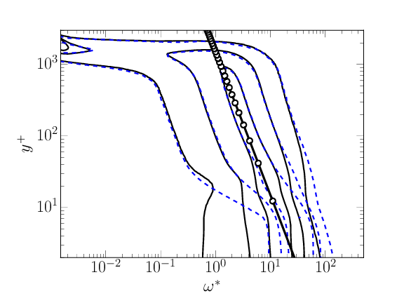
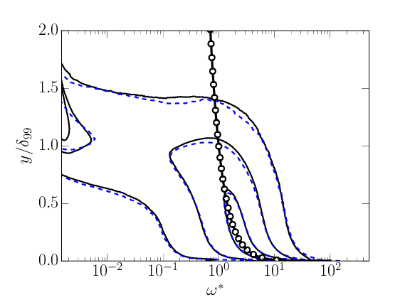
\( \omega^* \Gamma_{\omega^*,y}\) . Smooth: Dashed blue. Forced: Solid black. \( \omega^+ = \sqrt{\kappa y^+}\) ( \( - \circ -) \). Note that \( \omega^* \) includes \( u_\tau \).
From the T/NT interface.
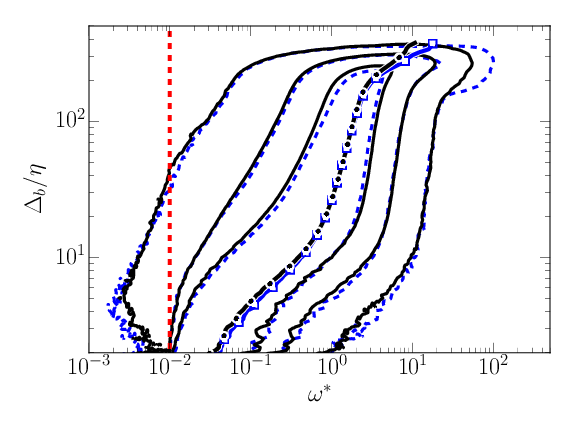
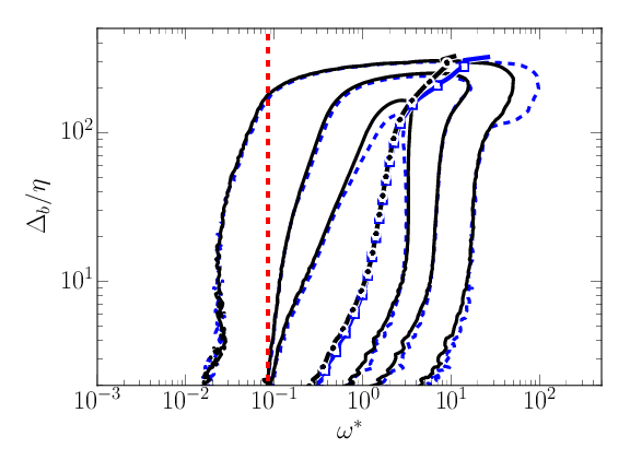
\( \omega^* F_{\omega^*,\Delta_b}\). Left: \( \omega_0^*=0.01 \). Right: \( \omega_0^* = 0.09 \). Smooth: Dashed blue, ( \( \overline{\omega}(\Delta_b), \color{blue}{\square} \) ). Forced: Solid black ( \( \overline{\omega}(\Delta_b), \bullet \) ). \( \omega = \omega_0 \) Red dashed
From the T/NT interface.
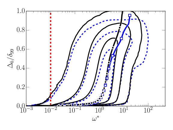
\( \omega^* F_{\omega^*,\Delta_b}\). Left: \( \omega_0^*=0.01 \). Right: \( \omega_0^* = 0.09 \). Smooth: Dashed blue, ( \( \overline{\omega}(\Delta_b), \color{blue}{\square} \) ). Forced: Solid black ( \( \overline{\omega}(\Delta_b), \bullet \) ). \( \omega = \omega_0 \) Red dashed
The effect of additional entrainment.
- \( \Delta_b \) recovers wall similarity.
- The forced boundary layer is intermittent.
- The structure of the turbulent flow is slightly different.
- The structural differences are encoded in the T/NT.
Conclusions
- Townsend's hypothesis:
- ✔One-point statistics.
- \( y/\delta_{99} \lesssim 0.2 \) → \(y \)
- \( y/\delta_{99} \gtrsim 0.2 \) → \(\Delta_b \)
- ✘Structural similarity.
- Even with a structure-less forcing.
- More friction → less intermittency.
- Entrainment:
- Contained within a thin T/NT layer.
- Entrainment rate similar with \( \omega^* \).
- Small-scale process (nibbling).
THE END
Questions?
Backup slides
Fractal Dimension
\( N_b \) the number of boxes of size \( r \) that cover \( \Omega \)
\[ \dim_b=-\lim_{r\rightarrow \varsigma} \frac{ \log N_b}{\log r},\quad D_b(r)=-\frac{\mbox{d} \log N_b}{\mbox{d} \log r} \]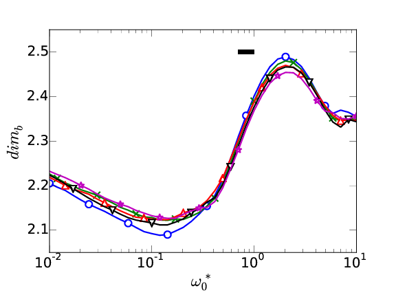
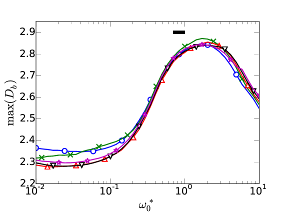
\( \delta_{99}^+= \color{blue}{1100}, \color{green}{1300}, \color{red}{1500}, \color{black}{1700}, \color{magenta}{1900} \)
Genus
The genus is a topological invariant of a connected surface equal to the number of handles on it. Evaluates the topological complexity of a surface.


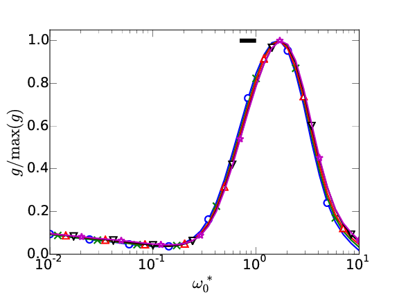
Geometrical complexity and \( \omega_0 \)
- The threshold as an important effect.
- There is a topological transition caused by the threhsold.
- The interface below \( \omega_0^* \sim 0.1 \) is smooth
- Above \( \omega_0^*=1 \) the geometrical properties of the fully turbulent flow characterize the interface.
- Good collapse for the two complexity measures with the Reynolds number if star units are used.
- Topological complexity is an issue for the conditional analysis.
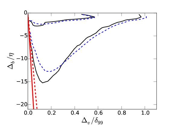
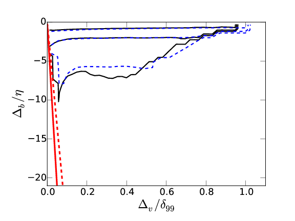
Distance field
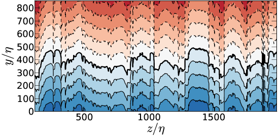
Top \( \Delta_b \), bottom \( \Delta_v \). Left \( \omega_0^*=0.01 \), right \( \omega_0^*=0.5 \)
Top \( \Delta_b \), bottom \( \Delta_v \). Left \(
\omega_0^*=0.01 \), right \( \omega_0^*=0.5 \).
Contours
=[50%, 90%, ~100%]
Top \( \Delta_b \), bottom \( \Delta_v \). Left \(
\omega_0^*=0.01 \), right \( \omega_0^*=0.5 \).
\(\overline{ \omega}
(\Delta) \): \( Q_1 + Q_2 \) \( \color{black}{\square}\), \(
Q_1\) \( \color{green}{\bigcirc} \), \( Q_2 \) \( \color{blue}{\triangle} \)
Handles, pockets and engulfment
The interior and handles, and pockets correspond to \( \Delta_b < 0 \) and \( \Delta_v > 0 \). Triple PDF of \( \omega^* \), \( \Delta_b \) and \( \Delta_v \)
Left: population (60% and 98%). Right: \( \overline{\omega} \) =[0.35,0.25,0.15] . \( \omega_0^*=0.5\ \). \( \delta_{99}^+=1100 \) (Solid), \( \delta_{99}^+=1900 \) (Dashed)
Strain
\( S = || \boldsymbol{\mathsf{S}} || \), \( \langle \omega ^2 \rangle = 2 \langle S^2\rangle \), \(S^* = S \nu \sqrt{2 \delta_{99}^+}/u_\tau \)
Left: \( \omega^*F_{\omega^*,y}\ (\color{blue}{-\ -}\color{black}{)} \), \( S^*F_{S^*,y}\ (\color{black}{-}) \)
Right: Strain interface ( \( \bigcirc \) ). Vorticity interface ( \( - \) ).